Influencing Factors on Conductivity Measurements on Conductivity Measurements
The accuracy of conductivity measurements is influenced by many factors most of which have been compensated for during the evolution of conductivity sensors.
Cable resistance and capacitance
Cable resistance is only an issue when working with two-pole sensor since in a four pole or six electrode sensor there is hardly any current flow via the voltage measuring electrodes that would be influenced by cable resistance. Cable capacitance needs to be taken into consideration even when working with four pole sensor. Especially at low conductivities the influence of the cable becomes relatively big and needs to be minimized e.g., by lowering the frequency of the applied current. Typical ranges for cable resistance and capacitance are 0…2000 Ω and 0…2000 pF.
Temperature
Since conductivity in liquids is usually increasing with increasing temperatures, all conductivity meters are equipped with a temperature compensation function. Conductivity standards available for a wide range of conductivities always come with a table showing the conductivity of the standard at several temperatures, see DIN EN 27888. Because of the strong dependency of electrical conductivity from temperature any conductivity sensor should have an integrated temperature sensor.
Temperature correction
While standard temperatures like 20 or 25 °C (68 or 77 °F) are used for calibrations with conductivity standards, the measurement of sample conductivity usually is performed at different temperatures. In order to compare actual and historic measurements, or comparing conductivities of different samples, it is common practice to recalculate the measured conductivity to a standard temperature, such as 20 or 25 °C – or none. Most conductivity meters and converters offer this function, where the user can select the required standard temperature. The measurements are then stored as temperature corrected values”.
However, this temperature standardization can be made in a limited temperature range, near the calibration and sample measurement temperature. A rule of thumb is calibration temperature +/- 5°C can be used for correction. Beyond this range a sample temperature adjustment (cooling / heating) or a new calibration must be performed – to keep the accurate measurement result.
Temperature compensation
Aqueous solutions change the conductivity with temperature. Most sample behavior can be characterized by a linear “temperature coefficient” α (%/°C). This coefficient has to be entered manually into the converter setup, where the temperature correction and compensation is calculated following the formula:
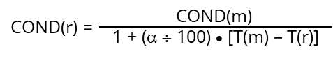
| COND(m) | conductivity measured at measurement temperature T(m) |
| COND(r) | conductivity calculated at reference temperature T(r) |
| T(m) | measurement temperature (°C) |
| T(r) | reference temperature (°C) |
| α | temperature coefficient (%/°C) |
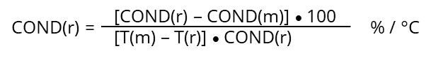
If the temperature coefficient of the specific sample is not known, it can be determined experimentally measuring the sample at reference temperature T(r) = 25°C and at second temperature T(m) like 15 or 35 °C (difference of 10°C or more).
For “natural waters” (6…100 mS/m) those “non-linear” temperature coefficients are listed in DIN EN 27888. In case existing conductivity results have been measured at 20°C they can be recalculated to 25°C by multiplying with the factor 1.116.
Polarization
Applying an electrical current to electrodes in solution causes the formation of a layer of counter ions close at the electrodes surface resulting in an additional capacitive resistance. The influence of this capacitive resistance is minimized by applying an alternating current (AC) avoiding the formation of ion layers. Higher AC frequencies are applied when measuring high conductivities, where the polarization resistance is big compared to the solution resistance. At low conductivities low AC frequencies are applied, which are less influenced by the cable capacity. When using a four pole cell the polarization resistance has hardly any effect on the measurement.
Geometry and cell constant
The quotient d/A [cm-1] is traditionally known as cell-constant (K) describing the area of the electrical field used to determine the conductivity. With the electrode arrangements of modern conductivity sensors the cell constant can be calculated by given dimensions (theoretical cell constant), but the real electrode area and surface structure adds to a “real cell constant”, which must be determined indirectly by a calibration in conductivity standard solutions. The measurement cell volume around the conductivity cell influences the cell constant as well. That is why a calibration of the completely installed system must be performed, when a new conductivity sensor is used. One factor influencing the properties of the electrical field is the ion concentration in the solution. This is why most modern sensor-transmitter systems work with editable cell constants to adjust for a wide conductivity range (µS up to S), using conductivity sensors with different cell constants or based on range specific calibrations.
Durability / shelf-life of conductivity standard solutions
The commercially available conductivity standard solutions cover a wide range of conductivities. While solutions of higher conductivities > 1000 mS can compensate for little contaminations over time, lower conductivities can change their nominal values quickly, e.g., if exposed to ambient air. Therefore it is good laboratory and manufacturing practice (GLP / GMP) to carefully check any conductivity standard before use. Old solutions and those opened many times for calibrations should be replaced by new standard solutions to maintain a constant level of accurate calibrations.
Accuracy of conductivity standard solutions
As stated before, the shelf-life is critical to conductivity standards, especially with low nominal values in µS range. This is why norms like DIN EN 27888 describe conductivity standards and their temperature behavior. Potassium chloride solutions of 1, 0.1 and 0.01 molar solutions are commonly used, having conductivities of 111.8, 12.88, and 1.408 mS/cm at 25°C. Those high concentrated KCl salt solutions can be produced with a final accuracy of +/-0.5%. However, low conductivity standards like 147 or 25 µS/cm solutions can go up to 5% accuracy. The accuracy directly goes into the uncertainty calculation of the sample measurement. A higher accuracy better than that of the standard cannot be achieved in sample measurements.
CO2 effect
Electrical conductivity in solutions is strongly influenced by any additional ions and dissolved gases. Ambient air consists of nitrogen (N2), oxygen (O2), carbon dioxide (CO2) and other nobel gases in lower concentrations. While N2 and O2 do not “dissolve” chemically as ions in aqueous solutions, CO2 does. It forms the carbonic acid H2CO3, which dissociates into ions:

The contact between low conductivity standards and ambient air must be avoided, because the CO2 adds ions to the standard solutions and changes the nominal value. Experiments have shown that ultrapure water starting with 0.05 µS/cm pouring into a glass beaker raises up to 1 µS/cm within seconds and moves even higher over time. The equilibrium between CO2 in air and in the aqueous solution is the driving force. This is why any measurement below 50 µS/cm must be made in sealed measurement cells and below 10 µS/cm an inert protection gas, like nitrogen N2, must be used to keep any air out of the solution or measurement cell (purge). With low conductivities it is even better to measure the sample in a sealed “flow-through” cell.
Stirring the sample
If not measuring the sample inline or in a flow, it is recommended to have a slight stirring (e.g., by a magnetic stirrer), but don’t create a vortex introducing air into the solution (adding CO2 !).